ABFE¶

This document describes how to run a ABFE simulation using Deep Origin tools.

Prerequisites¶

We assume that you have prepared a protein, docked a ligand to it, and obtained a pose that you want to proceed with.

In this tutorial we will use a protein and ligand from the example dataset.

from deeporigin.drug_discovery import (
    ABFE,
    SystemPrep,
    PreparedSystem,
    ABFEParams,
    BRD_DATA_DIR,
    Protein,
    Ligand,
)

protein = Protein.from_file(BRD_DATA_DIR / "brd.pdb")
protein.sync()

ligand = Ligand.from_sdf(BRD_DATA_DIR / "brd-2.sdf")
ligand.sync()

For more details on how to get started, see Getting Started .

System Preparation¶

Before ABFE, you must turn your protein and docked ligand into a simulation-ready systems. This step is called system preparation.

For a single ligand (i.e., ABFE), system prep builds two solvated models:

1. Binding system — protein and ligand assembled in an explicit water box with ions. This is the complex used for the binding leg of ABFE.
2. Ligand solvation system — the same ligand alone in solvent, used for the solvation leg.

Along the way, Deep Origin System Prep typically:

• Cleans and standardizes the protein structure, optionally protonates it at physiological pH, and assigns a protein force field (default Amber ff14SB).
• Parameterizes the ligand (hydrogens, charges, GAFF2 or OpenFF), then merges it with the protein into a complex.
• Solvates each system (water box padding, salt, optional retention of crystal waters).

sysprep = SystemPrep(
    protein=protein,
    ligand=ligand,
)

system = sysprep.run()
system.show()

You will see something like:

Estimating costs¶

Before starting a ABFE run, you can estimate costs using:

abfe = ABFE(prepared_system=system)
abfe.start(quote=True)
abfe.estimate

You will get back an estimate (in USD) of how much this run will cost.

Starting an ABFE run¶

Confirming a quoted Job¶

To confirm the quoted price and start the execution, do:

abfe.confirm()

This will start the ABFE run. Use the following to monitor the status of the job:

task = await abfe.watch()

You will see a widget similar to this (progress simulated for demonstration):

Parameters¶

ABFE simulation parameters are controlled via the ABFEParams dataclass. Default values are tuned for production runs; most users will only need to adjust a small number of fields.

Viewing parameters¶

To inspect the current parameters on an ABFE object, access the params property:

abfe.params

ABFEParams(
  annihilate: True
  dt: 0.004
  temperature: 298.15
  cutoff: 0.9
  repeats: 3 *
  replex_period_ps: 2.5
  test_run: 0
  binding_n_windows: 48
  binding_npt_reduce_restraints_ns: 2.0
  binding_nvt_heating_ns: 1.0
  binding_steps: 1250000
  solvation_n_windows: 32
  solvation_npt_reduce_restraints_ns: 0.2
  solvation_nvt_heating_ns: 0.1
  solvation_steps: 500000
)

Modifying parameters¶

ABFEParams is a frozen dataclass. Use dataclasses.replace() to build a modified copy and pass it to the constructor:

from deeporigin.drug_discovery import ABFEParams
from dataclasses import replace

params = replace(ABFEParams(), repeats=3, temperature=300)
params

Parameters modified from the defaults are indicated with an asterisk:

ABFEParams(
  annihilate: True
  dt: 0.004
  temperature: 300 *
  cutoff: 0.9
  repeats: 3 *
  replex_period_ps: 2.5
  binding_n_windows: 48
  binding_npt_reduce_restraints_ns: 2.0
  binding_nvt_heating_ns: 1.0
  binding_steps: 1250000
  solvation_n_windows: 32
  solvation_npt_reduce_restraints_ns: 0.2
  solvation_nvt_heating_ns: 0.1
  solvation_steps: 500000
)

Results¶

Viewing results¶

After a run completes successfully, fetch results with:

df = abfe.get_results()
df

This shows a table similar to:

Viewing trajectories¶

To view MD trajectories from this run, refer to ABFE.

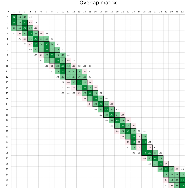
Viewing overlap matrix¶

An FEP overlap matrix is a diagnostic used in free energy perturbation calculations to evaluate how well neighboring λ states sample overlapping regions of configuration space. Each matrix element measures the statistical overlap between configurations from different states based on their energy distributions. The goal is to ensure every state has overlap with its neighbors in both directions – so that off-diagonal elements are sufficiently larger than zero.

The plot path is read from the data-platform result for this execution (default repeat=1, same indexing as abfe.show_trajectory). In Jupyter:

abfe.show_overlap_matrix(run="binding")

An image such as the following will be shown:

To view the overlap matrix for the solvation leg:

abfe.show_overlap_matrix(run="solvation")

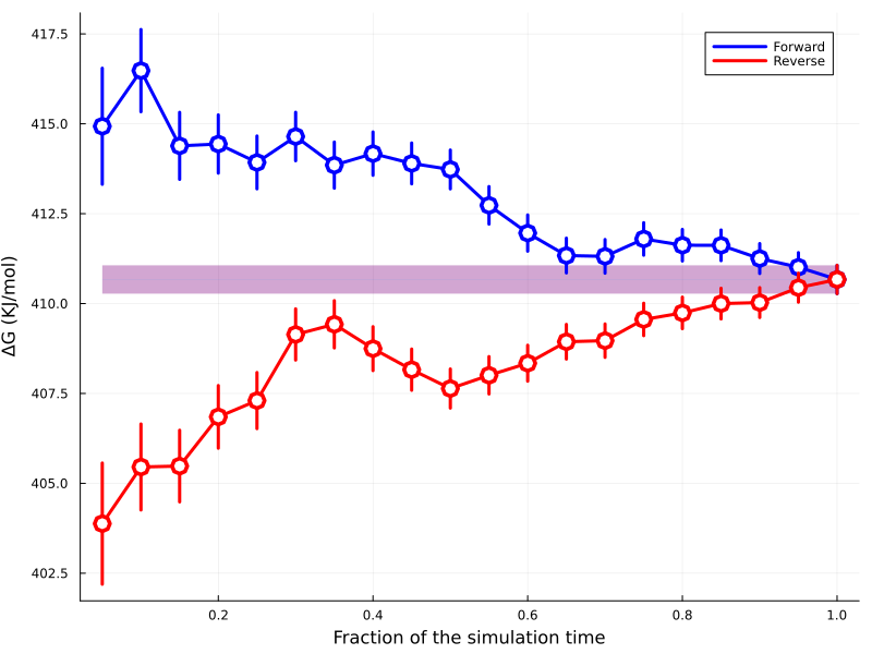
Viewing convergence time plots¶

The time-convergence diagnostic (convergence_plot in the result payload) can be shown the same way as the overlap matrix (default repeat=1, same as abfe.show_overlap_matrix and abfe.show_trajectory):

abfe.show_convergence_time(run="binding")

An image such as the following will be shown:

For the solvation leg:

abfe.show_convergence_time(run="solvation")